Stern-Gerlach Experiments

References

• “Quantum Mechanics”, Daivd McIntyre

In 1922, Otto Stern and Walther Gerlach performed a seminal experiment in the history of Quantum mechanics. It consisted of an overn that produced a beam of neutral Silver atoms, a region of space with an inhomogeneous magnetic field, and a detector for the atoms. Stern and Gerlach found that the beam was split in two in its passage through the magnetic field. One beam was deflected upwards and one downwards in relation to the direction of the magnetic field gradient.

We expect such behaviors from a neutral particle if it possesses a magnetic moment $\mu$. The potential energy of this interaction is $E=-\vec{\mu }\cdot \vec{B}$, which results in a force $\vec{F}=\nabla (\vec{\mu }\cdot \vec{B})$. In the experiment, the magnetic field gradient is primarily in the z-direction, and the resulting z-component of force is

$$F_z=\frac{\partial }{\partial z}(\vec{\mu }\cdot \vec{B})={\mu }_z\frac{\partial B_z}{\partial z}$$

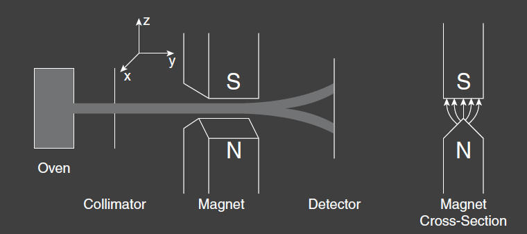
The force is perpendicular to the direction of motion and deflects the beam in proportion to the component of the magnetic moment in the direction of the magnetic field gradient.

Consider how the atom’s magnetic moment arises from a classical viewpoint. The atom consists of charged particles, which, if in motion, can produce loops of current that give rise to magnetic moments. A loop of area A and current I produces a magnetic moment

$$\mu =IA$$

in MKS units. If this loop of current arises from a charge q traveling at a speed v in a circle of radius r, then

$$\mu =\frac{q}{2\pi r/v}\pi r^2=\frac{qrv}{2}=\frac{q}{2m}\vec{L}$$

where $L=mrv$ is the orbital angular momentum of the particle. In the same way that earth revolves around the sun and rotates around its own axis, we can also imagine a charged particle in an atom having orbital angular momentum L and a new property, the intrinsic angular momentum, which we label $\mathbf{S}$ and call spin.

This intrinsic angular momentum also creates current loops, so we expect a similar relation between the magnetic moment $\vec{\mu }$ and $\vec{S}$. The exact calculation involves an integral over the charge distribution. We simply assume that we can relate the magnetic moment to the intrinsic angular momentum giving

$$\vec{\mu }=g\frac{q}{2m}\vec{S}$$

where the dimensionless gyroscopic ratio $g$ contains the details of the integral.

A silver atom has 47 electrons, 47 protons, and 60 or 62 neutrons. The magnetic moment is inversely proportional to the particle’s mass, so we expect the heavy protons and neutrons to have little effect on the magnetic moment of the atom so we neglect them. The Silver atom has electron configuration $1s^{2}2s^{2}2p^{6}3s^{2}3p^{6}4s^{2}3d^{10}4p^{6}4d^{10}5s^1$, which means there is only the lone 5s electron outside closed shells. Electrons in closed shells can be represented by a spherically symmetric cloud with no orbital or intrinsic angular momentum. That leaves the lone 5s electron as a contributor to the magnetic moment of the atom as a whole. An electron in an s state has no angular momentum, but it does have spin. Hence the magnetic moment of this electron, and therefore of the entire neutral silver atom is

$$\vec{\mu }=-g\frac{e}{2m_e}\vec{S}$$

where $e$ is the magnitude of the electron charge. The classical force on the atom can now be written as

$$F_z=-g\frac{e}{2m_e}{S}_z\frac{\partial B_z}{\partial z}$$

The deflection of the beam in the Stern-Gerlach experiment is thus a measure of the component (or projection) $S_z$ of the spin along the z-axis, which is the orientation of the magnetic field gradient.

If we assume that the 5s electron of each atom has the same magnitude $|\vec{S}|$ of the intrinsic angular momentum or spin, then classically we would write the z-component as $S_z=|\vec{S}|\cos \theta$, where $\theta$ is the angle between the z-axis and the direction of the spin $\vec{S}$. In the thermal environment of the oven, we expect a random distribution of spin direction and hence all possible angles $\theta$. Thus we expect some continuous distribution (details not important) of spin components from $S_z=-|\vec{S}|$ to $S_Z=+|\vec{S}|$, which would yield a continuous spread in deflections of the silver atomic beam. Rather, the experimental result is that there were only two deflections, indicating that there are only two possible values of the z-component of the electron spin. The magnitudes of these deflections are consistent with values of the spin component of

$$S_z=\pm \frac{\hslash }{2}$$

where $\hslash$ is Planck’s constant $h$ divided by $2\pi$ and has the numerical value

$$\hslash =1.0546\times 10^{-34}\mathrm{J}\cdot \mathrm{s}=6.5821\times 10^{-16}\mathrm{eV}\cdot \mathrm{s}$$

The result of the SG-experiment is evidence of the quantization of the electron’s spin angular momentum along an axis. We could have chose any axis, there is nothing special about the z-axis. The factor of 1/2 in $S_z=\pm \frac{\hslash }{2}$ leads us to refer to this as a spin-1/2 system. The two possible results of spin are called spin up and spin down. The physical quantity being measured, like $S_z$ is called an observable.

In the figure above , the SG-device is labeled with the axis along which the magnetic field is oriented. The up and down arrows indicate the two possible measurement results for the device, $S_z=\pm \frac{\hslash }{2}$ when the field is oriented along the z-axis. This device is called an analyzer.

The input and output beams are labeled with a new symbol called a ket. A ket is a representation of a quantum state. They are mathematical expressions and represent all the information that we can know about that state. A ket $|+⟩$ is the quantum state of the atoms that exit the upper port corresponding to $S_z=+\hslash /2$. A ket $|-⟩$ is the quantum state of the atoms leaving the lower port corresponding to $S_z=-\hslash /2$. The input beam is labeled with the more generic ket $|\psi ⟩$. The symbol within the brackets is any simple label to distinguish the ket from other kets. The kets $|+⟩$, $|+\hslash /2⟩$. $|S_z=+\hslash /2⟩$, $|\hat{z}⟩$ are all equivalent ways of writing the same thing, in this case signifying that we have measured the z-component of the spin and it is spin up. The let $|\pm ⟩$ refers to both the $|+⟩$, and the $|-⟩$ kets. The ket notation was developed by Paul A.M. Dirac and is central to the approach to quantum mechanics.

Postulate 1

The state of a quantum mechanical system, including all the information you can know about it, is represented mathematically by a normalized ket $|\psi ⟩$

Experiment 1

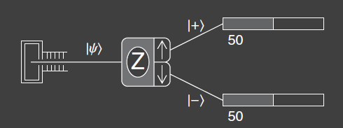
Experiment 1 consists of a source of atoms, two SG-analyzers both aligned along the z-axis, and counters for the output ports of the analyzers. The atomic beam coming into the first SG-analyzer is split into two beams at the output, just like the original experiment. Instead of counting the beams at the upper output port, they are sent to a second analyzer to measure the z-component of spin again. The first analyzer prepares the beam in a particular quantum state $|\pm ⟩$, and the second analyzer measures the resultant beam, so we often refer to the first analyzer as a state preparation device. By preparing the state, the details of the source of atoms can be ignored. The main focus is what happens at analyzer 2.

The result of the experiment is that all atoms that are output from the upper port of the first analyzer also pass through the upper port of the second analyzer. Thus we say that when the first SG-analyzer measures an atom to have a z-component of spin $S_z=+\hslash /2$, then the second analyzer also measures $S_z=+\hslash /2$ for that atom.

Experiment 2

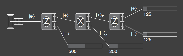
The second experiment is identical to experiment 1 except that the second SG-analyzer has been rotated 90 degrees to be aligned with the x-axis. Now the second analyzer measures the spin component along the x-axis rather than the z-axis. The atoms exiting the upper port are prepared in the $|+⟩$ state. The result of this experiment is that atoms appear at both possible output ports of the second analyzer, with spin components $S_x=\pm \hslash /2$. On average, each of these ports has 50% of the atoms that left the upper port of the first analyzer. The output states of the second analyzer have new labels ${|+⟩}_x$ and ${|-⟩}_x$, where x subscript denotes that the spin component has been measured along the x-axis. We assume that no subscript means we are talking about the spin component along the z-axis.

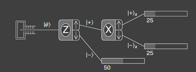
The experiment wouldn’t have turned out any differently if we would have used atoms output from the lower port of the first analyzer. We cannot predict which of the second analyzer output ports any particular atom will come out. This can be demonstrated in actual experiments by recording the individual counts out of each port. The arrival sequences at any counter are completely random. We can only say that there is a 50% probability that an atom from the second analyzer will exit the upper analyzer port and a 50% probability that it will exit the lower port.

This probabilistic nature is at the heart of quantum mechanics. One might be tempted to say that we just don’t know enough about the system to predict which port the atom will exit. That is to say, there may be some other variables, of which we are ignorant, that would allow us to predict the results. Such a viewpoint is known as a local hidden variable theory. John Bell proved that such theories are not compatible with the experimental results of quantum mechanics. The conclusion to draw from this is that even though quantum mechanics is a probabilistic theory, it is a complete description of reality.

Experiment 3

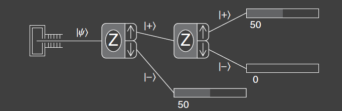
Experiment 3 extends Experiment 2 by adding a third SG-analyzer aligned along the z-axis. Atoms entering the third analyzer have been measured by the first SG-analyzer to have spin component up along the z-axis, and by the second analyzer to have spin component up along the x-axis. The third analyzer then measures how many atoms have spin component up or down along the z-axis. Classically, one would expect that the final measurement would yield the result spin up along the z-axis, because that was measured at the first analyzer. The first two analyzer tell us that the atoms have $S_z=+\hslash /2$ and $S_x=+\hslash /2$, so the third measurement must yield $S_z=+\hslash /2$. But that doesn’t happen, the quantum mechanical result is that the atoms are split with 50% probability into each output port at the third analyzer. Thus, the last two analyzers behave like the two analyzers of experiment (order reversed), and the fact that there was an initial measurement that yielded $S_z=+\hslash /2$ is somehow forgotten or erased.

This result demonstrates another feature of quantum mechanics: a measurement disturbs the system. The second analyzer has disturbed the system such that the spin component along the z-axis does not have a unique value, even though we measured it with the first analyzer. One could ask, can I be more clever in designing the experiment such that I don’t disturb the system? The short answer is no. There is a fundamental incompatibility in trying to measure the spin component of the atom along two different directions. So we say that $S_z$ and $S_x$ are \textbf{incompatible observables}. We cannot know the measured values of both simultaneously. The state of the system can be represented by the ket $|+⟩=|S_z=+\hslash /2⟩$ or by the ket ${|+⟩}_x=|S_x=+\hslash /2⟩$, but it cannot be represented by a ket $|S_z=+\hslash /2,S_x=+\hslash /2⟩$ that specifies the values of both components. It should be said however that not all pairs of quantum mechanical observables are incompatible. It is possible to do some experiments without disturbing some of the other aspects of the system.

Not being able to measure both $S_z$ and $S_x$ spin components is clearly distinct from the classical case where we can measure all three components of the spin vector, which tells us which direction the spin is pointing. In quantum mechanics, the incompatibility of the spin components means that we cannot know which direction the spin is pointing. So when we say “the spin is up” we really mean only that component along that one axis is up. The quantum mechanical spin vector cannot said to be pointing in any given direction.

Experiment 4

In experiment 4c, two output beams are combined as input to the following analyzer. This is simple in principle but can be difficult in practice. The recombination of the beams bust be done properly so as to avoid “disturbing” the beams. More information on this in Feynmann’s Lectures on Physics, volume 3. Experiment 4a is identical to Experiment 3. Experiment 4b is different in that the upper beam of the second analyzer is blocked and the lower beam is sent to the third analyzer. It should be clear from our previous experiments that Experiment 4b has the same results as Experiment 4a.

We now ask about the results of experiment 4c. If we were to use classical probability analysis, then Experiment 4a wold indicate that the probability for an atom leaving the first analyzer to take the upper path through the second analyzer and then exit through the upper port of the third analyzer is 25%, where we are now referring to the total probability for those two steps. Likewise, for Experiment 4b. Hence the total probability to exit from the upper port of the third analyzer when both paths are available, in Experiment 4c, would be 50%, and likewise for the exit from the lower port.

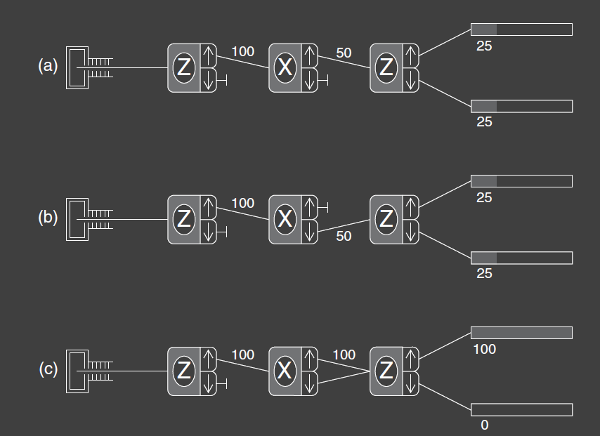
However the quantum mechanical result in Exp 4c is that all the atoms exit the upper port of the third analyzer and none exits the lower port. The atoms now appear to “remember” that they were initially measured to have spin up along the z-axis. By combining the two beams from the second analyzer, we have avoided the quantum mechanical disturbance that was evident in Exp 3, 4a, and 4b. The result is now the same as Exp 1, which means it as if the second analyzer is not there.

To see how odd this is, look carefully what happens at the lower port of the third analyzer. In this discussion, we refer to percentages of atoms leaving the first analyzer, because that analyzer is the same in all three experiments. In Exp 4a and 4b, 50% of the atoms are blocked after the middle analyzer and 25% of the atoms exit the lower port of the third analyzer. In Exp 4c , 100% of the atoms pass from the second analyzer, yet fewer atoms come out of the lower port. In fact, no atoms make it through the lower port! So we have a situation where allowing more ways or paths to reach the counter results in fewer counts. Classical probability theory cannot explain this aspect of quantum mechanics. It is as if you opened a second window in a room to get more sunlight and the room went dark!

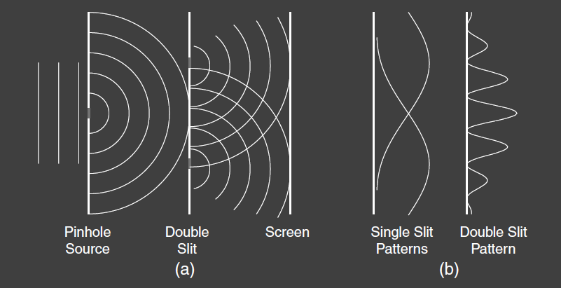
Imagine a procedure whereby combining two effects leads to cancellation rather than enhancement. The concept of wave interference, especially in optics, comes to mind. In the Young’s double-slit experiment, light waves pass through two narrow slits and create an interference pattern on a distant screen, as in Fig 7. Either slit by itself produces a nearly uniform illumination of the screen, but the two slits combined produce bright and dark interference fringes, as shown in Fig 7 (b). We explain this by adding together the electric field vectors of the light from the two slits, then squaring the resultant vector to find the light intensity. We say that we add the amplitudes and then square the total amplitude to find the light intensity.

We follow a similar prescription in quantum mechanics. We add together amplitudes and then take the square to find the resultant probability, which opens the door to interference effects. Before we discuss quantum mechanical interference, we must explain what we mean by an amplitude and how to calculate it.